Kalman filter and pair trading

Pair trading is a type of cointegration approach to statistical arbitrage trading strategy in which usually a pair of stocks are tcraded in a market-neutral strategy, i.e. it doesn’t matter whether the market is trending upwards or downwards, the two open positions for each stock hedge against each other. The key challenges in pairs trading are to:

• Choose a pair which will give you good statistical arbitrage opportunities over time
• Choose the entry/exit points

One of the challenges with the pair trading is that cointegration relationships are seldom static. I implemented a Kalman filter to track changes in this relationship between the stocks with synthesized stocks data.

data sythesis

These are some initil paramaters for octabe/matlab simulation:

mu=0.1;
t=1:1000;
sig=0.3;
T=1;
N=1000;
r=mu-sig^2/2;
Y=randn;
h=T/N;
sh=sqrt(h);
mh=r*h;
x0=100;

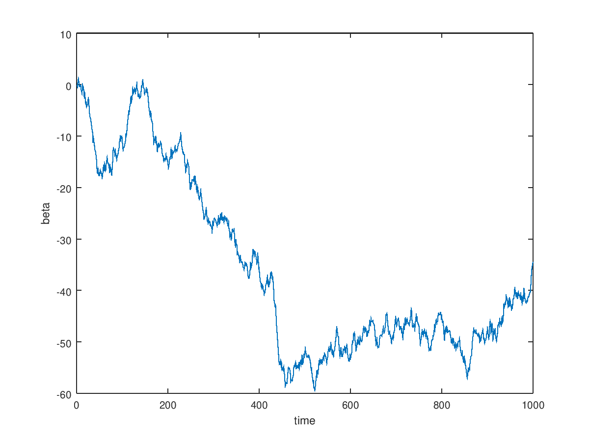
I have used the simplest form to model the relationship between a pair of securities in the following way: $$ \beta(t) = \beta(t-1) + \omega\\ \omega \sim N(0,Q)\\ $$ where beta is the unobserved state variable that follows a random walk, and W is a Gaussian distributed process with men 0 standard deviation Q.

R=sqrt (0.001);
Q=sqrt(0.00001);
beta=1+cumsum (Q*randn(size(t)));

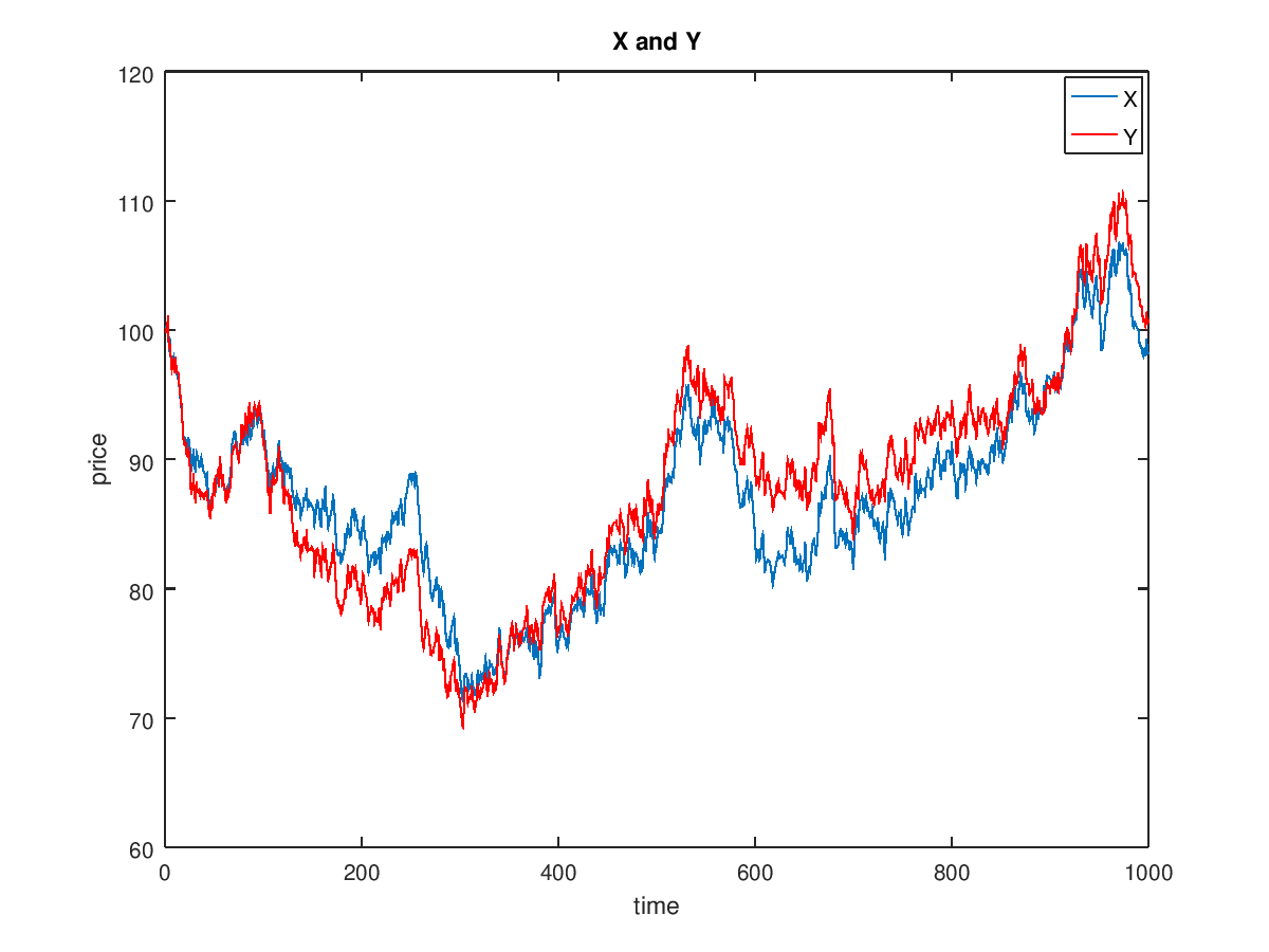
The observed processes of stock prices Y(t) and X(t) and V is gaussion disribued process with men 0 standard deviation R. $$ Y(t)=\beta(t)X(t)+v \\ v \sim N(0,R)\\ $$

clear G
X=x0;
G(:,1)=[0 x0];
for j=2:N
	z=randn;
	X=X*exp(mh+sh*sig*z);
	G(:,j) = [j*h X];
end
x=G(2,:);
y=x.*beta + R*randn(size(t));

Kalman filer

Instead of the typical approach to estimate beta using least squares regression, or some kind of rolling regression (to try to take account of the fact that beta may change over time). In this traditional framework, beta is static or slowly changing.
In the Kalman framework, beta is itself a random process that evolves continuously over time, as a random walk. Because it is random and contaminated by the noise, we cannot observe beta directly but must infer its (changing) value from the observable stock prices X and Y.
Kalman filter has very complicated mathematical and statistical theory behind it. See here for tutorial. Kalman filter algorithm has two states:

• prediction: in this stage, the algorithm will predict the next beta before it has the stock prices. The prediction is at time t and based on beta values from previous times.
• update: in this stage, the algorithm will update the prediction of beta after it has the stock price at time t.

Q=0.8;
H=1;
P=1;
K=1;
F=[0.1  0.1 .8  ];n=3;
beta_est(1:n)=beta(1:n);
clear PP
for i=n+1:size(t,2)
	%Prediction
	beta_est(i)=F*beta_est(i-n:i-1)';
        P=F*P*F'+Q;

       % uses to decide for trade since index 'i'  is a later time, and we have info till time 'i-1'.
	beta_pred(i)=F*beta_est(i-n:i-1)';
	

	% update , it time 'i' and the stock info at this time is known
	r= y(i)/x(i) -beta_est(i);
	K=P^1*H'*(R+H*P^-1*H')^-1;
	beta_est(i)=beta_est(i) + K*r;
	P=(ones(1,1)-K*H)*P;
	PP(end+1,:) = [P K];	
end

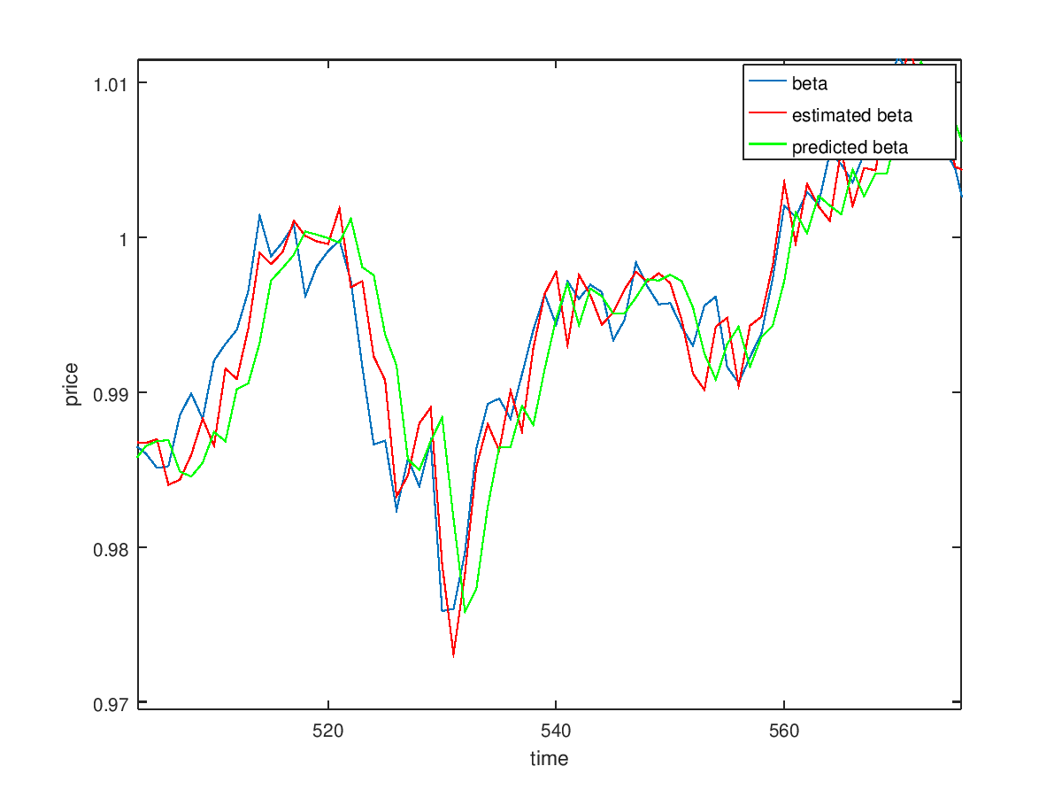
The following figure diplaye kalman filter resolt. The blue graph is the orignal beta, which is hidden variable and cannot diplayed directly. The green one is the preidcted beta which is used by the trade algorithm to take descitiopn about trade. The red graph is estimated beta which calculated right after the update stage.

trading algorithm

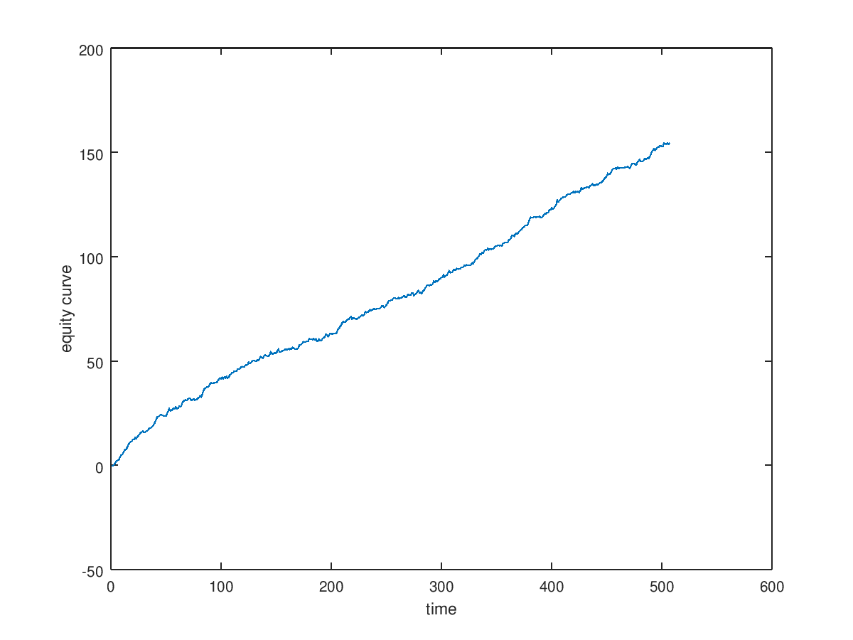
The trading algorithm is very simple and show great resoluts: $$ position(t)=\left\{ \begin{array}{ll} 1 & , beta>0 \\ -1 & , beta<0 \end{array} \right. $$

ii=find  (y-beta_pred.*x>0.0);
s=y- beta_pred.*x;
s=[0 diff(s)];
ii=ii(10:end); % ignore the converegance time of kalman filter
figure;plot (cumsum(s(ii)))
xlabel('time');
ylabel('equity curve');

conclusions

The results above are only theoretical and to apply this approach to real stock there arise a lot todo:

1. to find a cointegrated pair of stocks.
2. to find an automatic way to calibrate the Kalman-filter Q parameter.
3. find a more complicated trading algorithm. For example: train a neural network model to get a maximum equity curve with maximum share ration.
4. One can choose a better relationship model between stocks of the pair.
5. The above equity curve is theoretical only since the synthesized data is stationary, and therefor the equity curve continuously grows. In a real stock pairing, the information is a complete mess, and the statistical characteristics are not known and not stationary. Nevertheless, it seems that the Kalman filter does an outstanding job with beta tracking and has a very high potential to work in the real trading strategy.

The code for this example is written in Matlab/octave and can be found here.

References

[1] http://jonathankinlay.com/2018/09/statistical-arbitrage-using-kalman-filter/
[2] https://www.intechopen.com/books/introduction-and-implementations-of-the-kalman-filter/introduction-to-kalman-filter-and-its-applications
[3] https://robotwealth.com/kalman-filter-pairs-trading-r/
[4] Algorithmic Trading: Winning Strategies and their Rationale, Wiley, 2013